In our previous discussions, we saw that \(R^2\), which was our measure of overall goodness-of-fit for linear regression models, really does not convey any relevant information for models like Logit
Furthermore, the usual t-tests, used to test hypotheses around \(\hat{\beta}\), is not applicable here
How can we test make hypothesis around Logit models and assess overall accuracy?
We’ll make use of the fact that Logit models are estimated using a likelihood function, \(\mathcal{L}\), in order to derive some important evaluation metrics
\[ \mathcal{L_i}(\beta,y_i,x_i)=[\Lambda(x_i\beta)^{y_i}]\times[1-\Lambda(x_i\beta)]^{1-y_i} \] Because we are assuming that all churn observations (i.e, al customer decisions) are i.i.d, then the likelihood of the entire sample is just the product of the individual likelihoods:
\[ \mathcal{L}(\beta,Y,X)=\prod_{i=1}^{N}[\Lambda(x_i\beta)^{y_i}]\times[1-\Lambda(x_i\beta)]^{1-y_i} \] - In words, a maximum-likelihood estimator is trying to find the coefficients \(\beta\) that make the sample of churn observations \((y_1,y_2,...,y_n)=Y\) more likely to occur!
What happens on the back-end is that a maximum likelihood estimator will try to find the set of parameters \(\beta\) that maximize the log-likelihood of the model, noting that the \(\log\) is a monotonic function
At the end of the day, when we want to compare models, we can think about which model has the highest log-likelihood
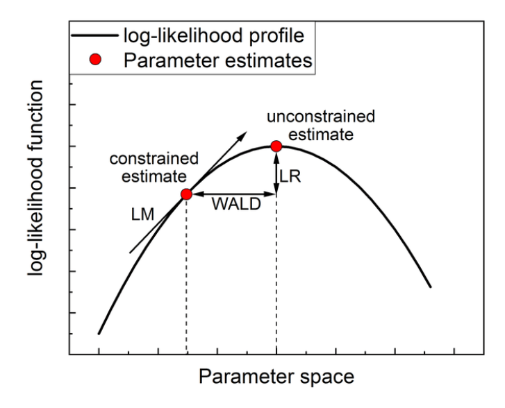
There are three common tests that can be used to test this type of question: the Likelihood ratio (LR) test, the Wald test, and the Lagrange multiplier test (sometimes called a score test)
These tests are sometimes described as tests for differences among nested models, because one of the models can be said to be nested within the other:

Wald Test for coefficient 1: 0
Wald Test for coefficient 2: 0.018847479056042
Wald Test for coefficient 3: 0
Wald Test for coefficient 4: 0
Wald Test for coefficient 5: 0.112919903979029
Wald Test for coefficient 6: 0
Wald Test for coefficient 7: 0.435636315719163
Wald Test for coefficient 8: 0.621715294810002
Wald Test for coefficient 9: 0
Wald Test for coefficient 10: 0.289254821503594
Data=read.csv('Exercises/bank-dataset.csv')
Reg=glm(churn ~ credit_score + gender + age + tenure + balance + products_number + credit_card + active_member + estimated_salary,
family = binomial(link = "logit"),
data = Data)
for(i in 1:10){
message(glue('Wald Test for coefficient {i}: {wald.test(b=coef(Reg),Sigma = vcov(Reg),Terms = i)$result$chi[3]}'))
}import pandas as pd
import statsmodels.api as sm
from scipy.stats import chi2
# Read the CSV file into a DataFrame
data = pd.read_csv('Exercises/bank-dataset.csv')
# Convert 'gender' to dummy variables
data = pd.get_dummies(data, columns=['gender'], drop_first=True)
# Define the independent variables and the dependent variable
X = data[['credit_score', 'gender_Male', 'age', 'tenure', 'balance', 'products_number', 'credit_card', 'active_member', 'estimated_salary']]
y = data['churn']
# Add constant term to the independent variables
X = sm.add_constant(X)
# Fit logistic regression model
reg = sm.Logit(y, X).fit()
# Wald test for each coefficient
wald_stat = reg.params / reg.bse
p_values = 1 - chi2.cdf(wald_stat ** 2, 1)
# Print p-values one per line
for p_value in p_values:
print(p_value)Optimization terminated successfully.
Current function value: 0.435323
Iterations 6
Likelihood Ratio Test:
Chi-square: 1403.3298480589165
Degrees of freedom: 9.0
P-value: 1.474938498277411e-296
import pandas as pd
import statsmodels.api as sm
# Read the CSV file into a DataFrame
data = pd.read_csv('Exercises/bank-dataset.csv')
# Convert 'gender' to dummy variables
data = pd.get_dummies(data, columns=['gender'], drop_first=True)
# Define the independent variables and the dependent variable
X = data[['credit_score', 'gender_Male', 'age', 'tenure', 'balance', 'products_number', 'credit_card', 'active_member', 'estimated_salary']]
y = data['churn']
# Add constant term to the independent variables
X = sm.add_constant(X)
# Fit logistic regression model
reg = sm.Logit(y, X.astype('float')).fit()
# Perform likelihood ratio test (LRT)
lr_test = reg.llr
df = reg.df_model
p_value = reg.llr_pvalue
print("Likelihood Ratio Test:")
print("Chi-square:", lr_test)
print("Degrees of freedom:", df)
print("P-value:", p_value)\[ \text{pseudo-}R^2=1-(\mathcal{LL}_{FullModel}/\mathcal{LL}_{\beta=0}) \]
If your model doesn’t really predict the outcome better than the null model, and the statistic will be close to zero
Conversely, if the difference in log-likelihood is large, your test will approach 1
McFadden
0.1388091
import pandas as pd
import numpy as np
import statsmodels.api as sm
# Read the CSV file into a DataFrame
data = pd.read_csv('Exercises/bank-dataset.csv')
# Convert 'gender' to dummy variables
data = pd.get_dummies(data, columns=['gender'], drop_first=True)
# Define the independent variables and the dependent variable
X = data[['credit_score', 'gender_Male', 'age', 'tenure', 'balance', 'products_number', 'credit_card', 'active_member', 'estimated_salary']]
y = data['churn']
# Add constant term to the independent variables
X = sm.add_constant(X)
# Fit logistic regression model
reg = sm.Logit(y, X).fit()
# Calculate McFadden's pseudo R-squared
def pseudoR2(model):
L1 = model.llf
L0 = sm.Logit(y, sm.add_constant(np.ones_like(y))).fit().llf
return 1 - (L1 / L0)
pseudo_r2 = pseudoR2(reg)
print("McFadden's Pseudo R-squared:", pseudo_r2)How the estimated results compare to actual choices from customers?
From a practical perspective, one needs to map the estimated probabilities onto a categorization:
\[ \hat{Y}= \begin{cases} 1 \text{, if } p>p^\star\\ 0 \text{, if } p\leq p^\star \end{cases} \]
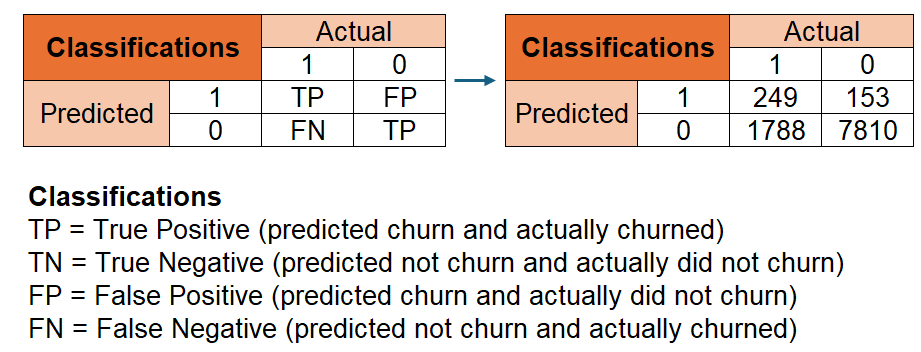
churn, our example would yield the following terms for us:
\[ \small ACC=\dfrac{TP+TN}{TP+FP+TN+FN}=\dfrac{1,387+5,486}{10,000}\approx 69\% \text{ correct predictions} \]
Notwithstanding, there might be cases where the costs attributed to Type I and Type II errors are fairly different!
The first question that will likely pop up during internal conversations is: how much of the churned customers we were able to correctly identify?
This question is of special interest in churn analysis, as the goal is to target these customers before they actually have their final decision!
The Sensivity (or the True Positive Rate) calculates the proportion of correctly identified churned customers by comparing the number of true positives with the total number of positives:
\[ Sensitivity=\dfrac{TP}{TP+FN}=\dfrac{1,387}{(1,387+650)}\approx 68\% \]
The naivest way of identifying all churned customers is to set \(p\star=0\). In other words, if we classify all customers as churned, then, for sure, we’ll get all churned customers right!
Notwithstanding, we are wrongly classifying some customers that would not churn in the future (false negatives). In practice, if we were to give coupons to every churn customer in potential, this action would cost us much more as we’re wasting money on customers that wouldn’t churn!
The Precision calculates the how precise our churn classification was by comparing the number of true positives with the total number of predicted positives:
\[ Precision=\dfrac{TP}{TP+FP}=\dfrac{1,387}{(1,387+2,477)}\approx 35\% \]
The analog of the first question relates to how much of the non-churned customers we were able to correctly identify
Knowing how much non-churned customers our model predicts shed light on how much we’re able to understand about customers that do not churn!
The Specificity (or True Negative Rate) calculates the proportion of correctly identified non-churned customers by comparing the number of true negatives with the total number of negatives:
\[ Specificity=\dfrac{TN}{TN+FP}=\dfrac{5,486}{(5,486+2,477)}\approx 69\% \]
The last piece that is still left to analyze is the precision of our estimates for non-churned classifications
In other words, out of all the non-churn predicted customers, how much were actually false negatives?
The Negative Predicted Value calculates the proportion of correctly identified non-churned customers by comparing the number of true negatives with the predicted negatives:
\[ NPV=\dfrac{TN}{TN+FN}=\dfrac{5,486}{(5,486+650)}\approx 89.37\% \]
Confusion Matrix and Statistics
Reference
Prediction 1 0
1 1387 2477
0 650 5486
Accuracy : 0.6873
95% CI : (0.6781, 0.6964)
No Information Rate : 0.7963
P-Value [Acc > NIR] : 1
Kappa : 0.2773
Mcnemar's Test P-Value : <2e-16
Sensitivity : 0.6809
Specificity : 0.6889
Pos Pred Value : 0.3590
Neg Pred Value : 0.8941
Prevalence : 0.2037
Detection Rate : 0.1387
Detection Prevalence : 0.3864
Balanced Accuracy : 0.6849
'Positive' Class : 1
Data=read.csv('Exercises/bank-dataset.csv')
Reg=glm(churn ~ credit_score + gender + age + tenure + balance + products_number + credit_card + active_member + estimated_salary,
family = binomial(link = "logit"),
data = Data)
#Creating a comparison between actual and predicted churn
Comparison=data.frame(Actual=Data$churn,
Predicted=ifelse(predict(Reg,type='response')>=mean(Data$churn),1,0))
#Create the confusion matrix using 1 (churn) as the (1,1) quadrant (full)
confusionMatrix(data=factor(Comparison$Predicted,levels=c(1,0)),
reference=factor(Comparison$Actual,levels=c(1,0)),
)import pandas as pd
import numpy as np
from sklearn.linear_model import LogisticRegression
from sklearn.metrics import ConfusionMatrixDisplay
from matplotlib import pyplot as plt
# Read the CSV file into a pandas DataFrame
Data = pd.read_csv('Exercises/bank-dataset.csv')
# Convert 'gender' into dummy variables
Data = pd.get_dummies(Data, columns=['gender'], drop_first=True)
# Define independent and dependent variables
X = Data[['credit_score', 'gender_Male', 'age', 'tenure', 'balance', 'products_number', 'credit_card', 'active_member', 'estimated_salary']]
y = Data['churn']
# Add a constant to the independent variables matrix for the intercept
X = sm.add_constant(X)
# Fit the linear regression model
model = sm.Logit(y, X.astype(float)).fit()
# Predict churn using the trained logistic regression model
predicted_churn = model.predict() >= y.mean() # Assuming a threshold of 0.5 for classification
# Convert predicted churn to binary (1 or 0)
predicted_churn = predicted_churn.astype(int)
# Create confusion matrix
ConfusionMatrixDisplay.from_predictions(y, predicted_churn)
plt.show()

Data=read.csv('Exercises/bank-dataset.csv')
Reg=glm(churn ~ credit_score + gender + age + tenure + balance + products_number + credit_card + active_member + estimated_salary,
family = binomial(link = "logit"),
data = Data)
#Creating a comparison between actual and predicted churn
Comparison=data.frame(Actual=Data$churn,
Predicted=ifelse(predict(Reg,type='response')>=mean(Data$churn),1,0))
Coords=coords(ROC,print.thres=TRUE)%>%mutate(metric=sensitivity+specificity)
Best=pull(coords(ROC,print.thres=TRUE,"best")[1])
Coords%>%
ggplot(aes(x=threshold,y=metric))+
geom_point()+
theme_minimal()+
labs(y='Specificity + Sensitivity',x='Threshold for churn assignment',
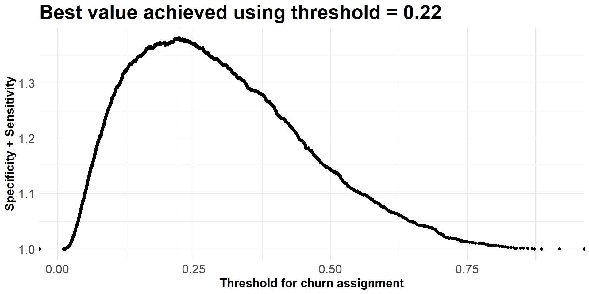
title=paste0('Best value achieved using threshold = ',round(Best,2)))+
geom_vline(xintercept = pull(coords(ROC,print.thres=TRUE,"best")[1]),linetype='dashed')+
theme(title=element_text(size=20,face='bold'),
axis.text = element_text(size=15),
axis.title = element_text(size=15))# Read the CSV file into a pandas DataFrame
Data = pd.read_csv('Exercises/bank-dataset.csv')
# Convert 'gender' into dummy variables
Data = pd.get_dummies(Data, columns=['gender'], drop_first=True)
# Define independent and dependent variables
X = Data[['credit_score', 'gender_Male', 'age', 'tenure', 'balance', 'products_number', 'credit_card', 'active_member', 'estimated_salary']]
y = Data['churn']
# Add a constant to the independent variables matrix for the intercept
X = sm.add_constant(X)
# Fit the linear regression model
model = sm.Logit(y, X.astype(float)).fit()
# Predict churn probabilities
probs = model.predict()
# Calculate specificity and sensitivity
fpr, tpr, thresholds = roc_curve(y, probs)
specificity = 1 - fpr
sensitivity = tpr
# Find the best threshold value
best_threshold_index = np.argmax(specificity + sensitivity)
best_threshold = thresholds[best_threshold_index]
# Visualize the results
plt.figure(figsize=(10, 6))
plt.plot(thresholds, sensitivity + specificity, marker='o')
plt.axvline(x=best_threshold, color='r', linestyle='--', label=f'Best Threshold: {best_threshold:.2f}')
plt.xlabel('Threshold for churn assignment')
plt.ylabel('Specificity + Sensitivity')
plt.title(f'Best value achieved using threshold = {best_threshold:.2f}')
plt.legend()
plt.grid(True)
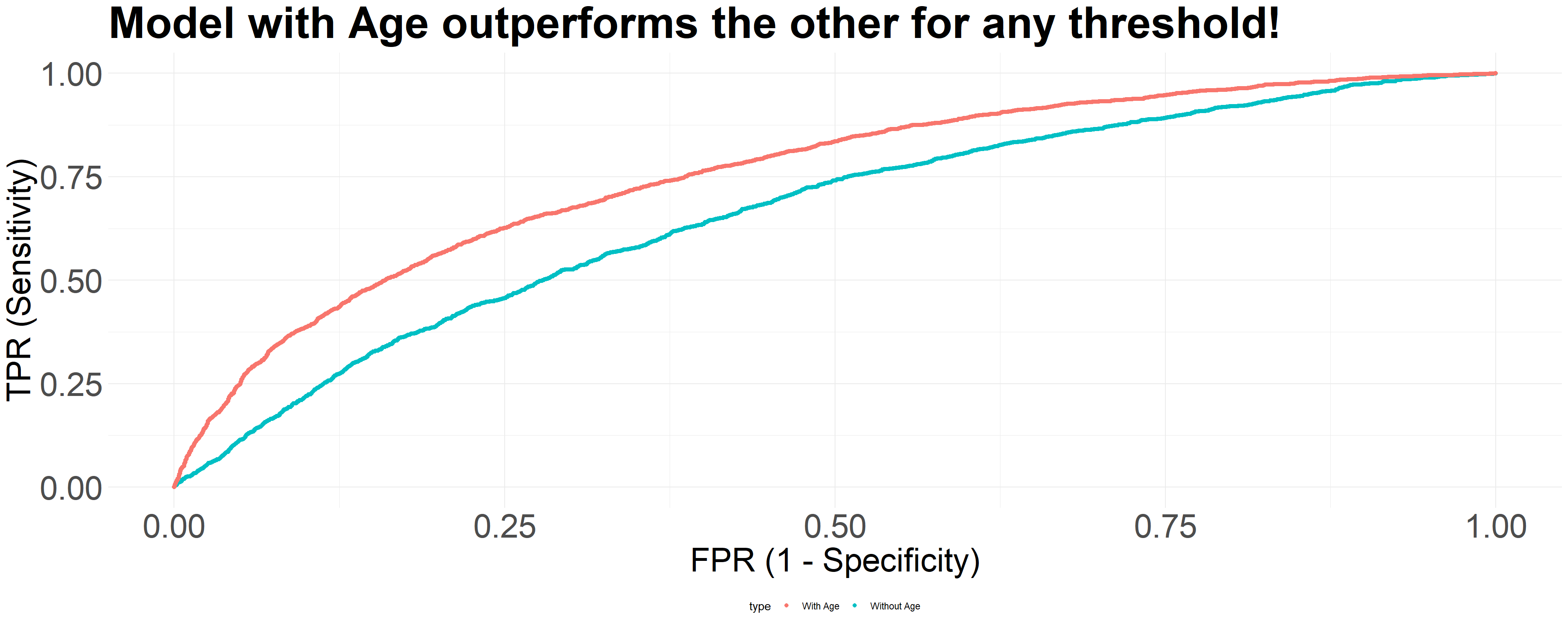
plt.show()age from the analysis. How can you assess how the predictive power of your model is going to deteriorate? One way to do this is to analyze what we call Area under the Curve (or simply AUC):
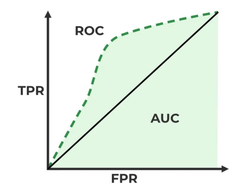
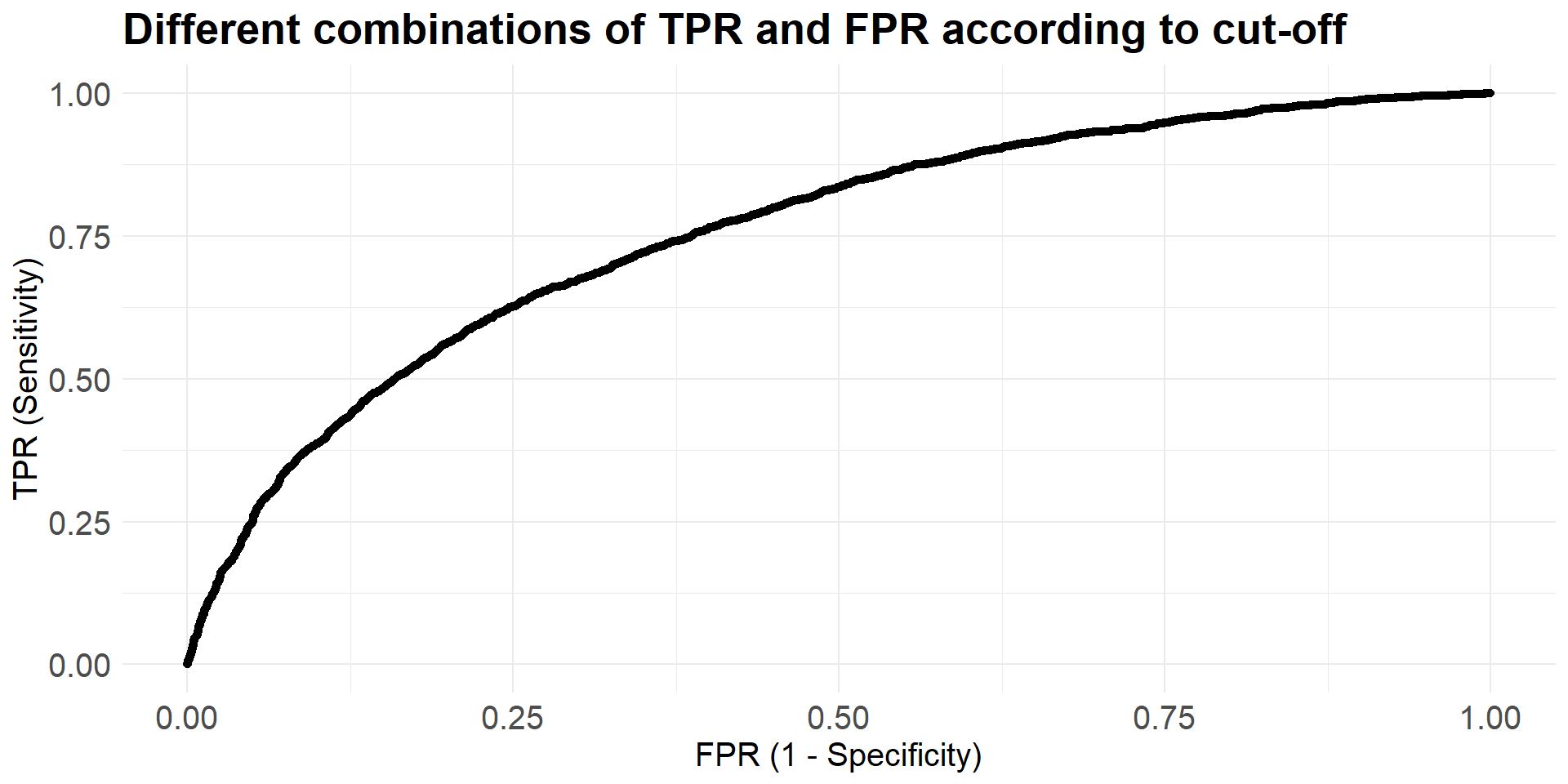
AUC provides an aggregate measure of performance across all possible classification thresholds
AUC isn’t a very useful metric whenever the costs of Type I and Type II errors are very different
Data=read.csv('Exercises/bank-dataset.csv')
Reg_1=glm(churn ~ credit_score + gender + tenure + balance + products_number + credit_card + active_member + estimated_salary,
family = binomial(link = "logit"),
data = Data)
Reg_2=glm(churn ~ credit_score + gender + age + tenure + balance + products_number + credit_card + active_member + estimated_salary,
family = binomial(link = "logit"),
data = Data)
P_1=Data%>%cbind(data.frame('Predicted'=predict(Reg_1,type='response')))
P_2=Data%>%cbind(data.frame('Predicted'=predict(Reg_2,type='response')))
ROC_1 = roc(P_1$churn ~ P_1$Predicted)
ROC_2 = roc(P_2$churn ~ P_2$Predicted)
ROC_1=coords(ROC_1)%>%mutate(TPR=sensitivity,FPR=1-specificity,type='Without Age')
ROC_2=coords(ROC_2)%>%mutate(TPR=sensitivity,FPR=1-specificity,type='With Age')
rbind(ROC_1,ROC_2)%>%
ggplot(aes(x=FPR,y=TPR,col=type))+
geom_point()+
theme_minimal()+
labs(x='FPR (1 - Specificity)',
y='TPR (Sensitivity)',
title='Model with Age outperforms the other for any threshold!')+
theme(plot.title = element_text(size=40,face='bold'),
axis.text = element_text(size=30),
axis.title = element_text(size=30),
legend.position ='bottom')import pandas as pd
import numpy as np
from sklearn.linear_model import LogisticRegression
from sklearn.metrics import roc_curve, roc_auc_score
import matplotlib.pyplot as plt
# Read the CSV file into a pandas DataFrame
Data = pd.read_csv('Exercises/bank-dataset.csv')
# Convert 'gender' into dummy variables
Data['gender'] = pd.get_dummies(Data['gender'], drop_first=True)
# Define independent and dependent variables for Reg_1 (without 'age')
X1 = Data[['credit_score', 'gender', 'tenure', 'balance', 'products_number', 'credit_card', 'active_member', 'estimated_salary']]
# Define independent and dependent variables for Reg_2 (with 'age')
X2 = Data[['credit_score', 'gender', 'age', 'tenure', 'balance', 'products_number', 'credit_card', 'active_member', 'estimated_salary']]
# Dependent variable
y = Data['churn']
# Fit logistic regression models
reg_1 = model = sm.Logit(y, X1.astype(float)).fit()
reg_2 = model = sm.Logit(y, X2.astype(float)).fit()
# Predict probabilities for both models
probs_1 = reg_1.predict()
probs_2 = reg_2.predict()
# Compute ROC curves
fpr_1, tpr_1, _ = roc_curve(y, probs_1)
fpr_2, tpr_2, _ = roc_curve(y, probs_2)
# Compute AUC scores
auc_1 = roc_auc_score(y, probs_1)
auc_2 = roc_auc_score(y, probs_2)
# Plot ROC curves
plt.figure(figsize=(10, 8))
plt.plot(fpr_1, tpr_1, color='blue', lw=2, label=f'Without Age (AUC = {auc_1:.2f})')
plt.plot(fpr_2, tpr_2, color='red', lw=2, label=f'With Age (AUC = {auc_2:.2f})')
plt.plot([0, 1], [0, 1], color='gray', lw=1, linestyle='--')
plt.xlim([0.0, 1.0])
plt.ylim([0.0, 1.05])
plt.xlabel('False Positive Rate (1 - Specificity)')
plt.ylabel('True Positive Rate (Sensitivity)')
plt.title('ROC Curve')
plt.legend(loc="lower right")
plt.show()There are some potential topics that you may want to dive in when looking at binary choice models (not only Logit):
Look for other binary classification models, such as Probit, Random Forests, etc
Bridging Econometrics with Machine Learning: there can be a variety of ways to make your analysis more robust:
R, refer to the caret package. For Python, refer to scikit-learn
Presented by Lucas S. Macoris